Normality test using SPSS: How to check whether data are normally distributed HD
If data need to be approximately normally distributed, this tutorial shows how to use SPSS to verify this. On a side note: my new project: http://howtowritecitations.com. Statistical analyses often have dependent variables and independent variables and many parametric statistical methods require that the dependent variable is approximately normally distributed for each category of the independent variable. Let us assume that we have a dependent variable, exam scores, and an independent variable, gender. In short, we must investigate the following numerical and visual outputs (and the tutorial shows how to do just that): -The Skewness & kurtosis z-values, which should be somewhere in the span -1.96 to +1.96; -The Shapiro-Wilk p-value, which should be above 0.05; -The Histograms, Normal Q-Q plots and Box plots, which should visually indicate that our data are approximately normally distributed. Remember that your data do not have to be perfectly normally distributed. The main thing is that they are approximately normally distributed, and that you check each category of the independent variable. (In our example, both male and female data.) Step 1. In the menu of SPSS, click on Analyze, select Descriptive Statistics and Explore. Step 2. Set exam scores as the dependent variable, and gender as the independent variable. Step 3. Click on Plots, select "Histogram" (you do not need "Stem-and-leaf") and select "Normality plots with tests" and click on Continue, then OK. Step 4. Start with skewness and kurtosis. The skewness and kurtosis measures should be as close to zero as possible, in SPSS. In reality, however, data are often skewed and kurtotic. A small departure from zero is therefore no problem, as long as the measures are not too large compare to their standard errors. As a consequence, you must divide the measure by its standard error, and you need to do this by hand, using a calculator. This will give you the z-value, which, as I said, should be somewhere within -1.96 to +1.96. Let us start with the males in our example. To calculate the skewness z-value, divide the skewness measure by its standard error. All z-values in the tutorial video are within ±1.96. We can conclude that the exam score data are a little skewed and kurtotic, for both males and females, but they do not differ significantly from normality. Step 5. Check the Shapiro-Wilk test statistic. The null hypothesis for this test of normality is that the data are normally distributed. The null hypothesis is rejected if the p-value is below 0.05. In SPSS output, the p-value is labeled "Sig". In our example, the p-values for males and females are above 0.05, so we keep the null hypothesis. The Shapiro-Wilk test thus indicates that our example data are approximately normally distributed. Step 6. Next, let us look at the graphical figures, for both male and female data. Inspect the histograms visually. They should have the approximate shape of a normal curve. Then, look at the normal Q-
Похожие видео
 HD
HD HD
HD HD
HD HD
HD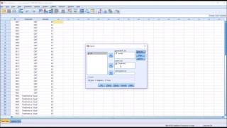 HD
HD HD
HD HD
HD HD
HD HD
HD HD
HD HD
HD![How To Check CPU Temp - The Easiest Way To Monitor GPU Temperature [BEGINNER'S TUTORIAL]](https://i.ytimg.com/vi/EfEFmKe9Cfo/mqdefault.jpg) HD
HD HD
HD HD
HD
 HD
HD HD
HD
 HD
HD HD
HD HD
HD HD
HD HD
HD HD
HD HD
HD
 HD
HD
 HD
HD HD
HD HD
HD HD
HDПоказать еще